Predicting and designing proteins (5): How inverse folding turned structures into sequences

17 Jul, 2026

Structure prediction asks what shape is compatible with a sequence. Protein design often asks the reverse question: which sequences are compatible with a desired shape? This reverse problem is called inverse folding. It sounds easier because the backbone is already supplied, but the answer is not unique. Many sequences can adopt similar folds, while small changes at a tightly packed core or binding interface can matter greatly.

Inverse folding became one of the most useful interfaces in computational design because it separates two kinds of work. A backbone generator can concentrate on the global geometry of a fold or interface. An inverse-folding model can then assign amino acids that fit the local environments. The final sequence can be encoded as DNA, synthesized, expressed by cells, and tested.

How classical design formulated the reverse problem

Rosetta-based design treated sequence choice as an energy optimization problem. For a fixed or partly flexible backbone, the algorithm selected side-chain identities and conformations, called rotamers, to improve an energy function. The calculation had to manage a combinatorial space: every position may accept several residue types, and every side chain may adopt several orientations.

For a supplied backbone $X,$ the calculation can be written schematically as

where $s$ is the amino-acid sequence, $r$ selects a rotamer at each designed position, and $E$ combines terms for packing, hydrogen bonding, electrostatics, solvation, and other modeled interactions. The notation $\mathrm{a}\mathrm{r}\mathrm{g}\mathrm{m}\mathrm{i}\mathrm{n}$ means “return the choices that give the smallest score,” not merely the value of that score.

A rotamer is one of the commonly observed ways a side chain can rotate around its chemical bonds. Even if a backbone is held still, choosing among twenty residue types and several rotamers at many positions produces an enormous number of combinations. The energy function is a computational scoring rule that approximates favourable packing and interactions; it is useful for comparing candidates, but it is not a direct experimental measurement of a molecule’s thermodynamic free energy.

This approach enabled landmarks such as Top7 and later idealized folds.¹² It also required substantial compute and expert decisions about which backbone movements, residue positions, and energy terms to permit. A hand-designed objective could favour the intended structure while missing alternative low-energy states, aggregation, or expression problems.

The growth of the PDB suggested a learned alternative. Every deposited protein supplies a training pair: its backbone geometry is the input, and its natural sequence is the target. A model can learn the conditional distribution “sequence given backbone” from many such examples.

Why proteins are represented as geometric graphs

A sequence is naturally a line, but a folded protein is a network of spatial neighbours. Residue 15 may contact residue 130 even though the two are distant along the chain. Graph neural networks represent residues as nodes and connect nearby residues with edges. Node features can describe residue position and local geometry; edge features can describe distances and relative orientations.

The graph is a bookkeeping device, not an additional biological structure. A node is simply the record associated with one residue, and an edge tells the network that two records should exchange information because the residues are nearby or otherwise relevant. Repeated message passing lets information travel beyond immediate neighbours: after several layers, a residue can be influenced by a larger region of the folded protein.

An inverse-folding model must also respect a basic symmetry: rotating or translating the whole protein should not change which sequences fit it. Geometric architectures therefore use invariant quantities, which remain unchanged under global motion, or equivariant quantities, which rotate in a predictable way with the structure.

John Ingraham, Vikas Garg, Regina Barzilay, and Tommi Jaakkola supplied an early learned formulation in 2019.³ Their model converted the backbone into a sparse graph, encoded the local coordinate system and relative geometry around each residue, and decoded the sequence autoregressively. The probability of a residue therefore depended on spatial neighbours and on residues already generated, including positions far away in the written chain but adjacent in the fold. This replaced repeated combinatorial rotamer search with learned conditional sampling, while retaining a limitation of autoregression: choices made early in the decoding order could constrain later choices.

Geometric vector perceptrons, introduced by Bowen Jing and colleagues, made the directional bookkeeping more explicit.⁴ Each node carried scalar channels, such as invariant chemical or positional features, and vector channels, such as directions associated with the backbone. A GVP layer mixes and gates these channels so that scalar outputs remain unchanged by a global rotation while vector outputs rotate with the protein. Stacking these layers let a network represent orientation without choosing an arbitrary global coordinate frame, and the construction became useful in both structure encoding and inverse folding.

If the vector channels are arranged as rows of a matrix $V$ and the whole structure is rotated by $R,$ this guarantee can be summarized as

The scalar result $s^{\prime }$ is unchanged, while every output vector in $V^{\prime }$ follows the rotation. Internally, vector norms such as $\Vert WV{\Vert }_2$ provide rotation-invariant numbers that can be mixed with ordinary scalar features; learned linear maps and gates then update the directional channels without tying the answer to one coordinate-file orientation.

ESM-IF1 joined that geometric encoder to a transformer decoder and addressed a different bottleneck: the limited number of experimentally determined structures.⁵ The team used AlphaFold2 to predict structures for 12 million protein sequences, increasing the structural training set by nearly three orders of magnitude. The encoder converted backbone coordinates into invariant geometric features; the decoder attended to those features while predicting amino acids. On structurally held-out backbones, the reported native-sequence recovery was 51%, rising to 72% for buried residues, whose tightly packed environments constrain their identities more strongly than solvent-exposed surfaces.

This scale-up carried an important trade-off. Predicted structures made many more folds available and helped the model transfer to complexes, masked regions, interfaces, and multistate design. They also imported AlphaFold2’s structural prior and confidence-dependent errors into the inverse-folding data. ESM-IF1 showed that predicted databases could become training corpora, not only end-user resources; ProteinMPNN showed how a smaller, deliberately robust graph model could become a dependable component of experimental design pipelines.

Why ProteinMPNN became a standard component

ProteinMPNN, developed by Justas Dauparas and colleagues in the Baker laboratory, made learned inverse folding fast, robust, and easy to insert into larger workflows.⁶ “MPNN” stands for message-passing neural network. Each residue updates its representation by exchanging messages with geometrical neighbours; the decoder then samples a sequence compatible with those accumulated environments.

Native-sequence recovery—the fraction of positions for which the model predicts the residue observed in nature—is a convenient benchmark, but it is not the final purpose. Natural sequences are only one solution, and sometimes not the best solution for a laboratory objective. More consequentially, ProteinMPNN-designed sequences expressed and folded successfully across diverse experimental projects. That prospective evidence helped establish it as more than a benchmark model.

ProteinMPNN also reduced design cost enough to make sampling routine. Designers can generate many sequences for one backbone at different sampling temperatures. A low temperature concentrates probability on conservative choices; a higher temperature explores more diversity. Positions can be fixed, tied by symmetry, or constrained to selected residue sets.

Sampling temperature is a mathematical control, not the temperature of a test tube. It reshapes the model’s probability distribution before a residue is drawn. Lower values magnify differences between high- and low-probability choices; higher values flatten those differences. The setting therefore controls exploration, but it cannot reveal whether a sampled sequence will be thermally stable in an experiment.

If the decoder assigns amino acid $a$ an unnormalized score, or logit, $z_a,$ sampling at temperature $\tau$ uses

As $\tau$ decreases, a small logit advantage becomes a much larger probability advantage. As $\tau$ increases, less-preferred residues receive more probability. The formula changes how the learned distribution is explored; it does not retrain the model or insert laboratory thermodynamics.

The resulting modular pipeline became common:

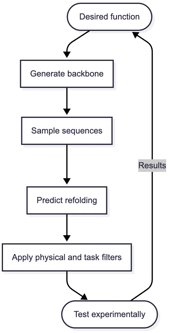
A backbone generator proposes geometry. ProteinMPNN proposes sequences. AlphaFold2, RoseTTAFold, or ESMFold tests whether each sequence is predicted to return to the intended geometry. Rosetta or specialized tools inspect packing, unsatisfied polar atoms, clashes, surface properties, and interfaces. A small set of candidates proceeds to experiment.

The modularity is operationally powerful, but it creates a subtle evidentiary problem. The generator, inverse folder, and structure predictor may all have learned related patterns from PDB-derived data. Their agreement is useful evidence of internal consistency, not three independent confirmations of physical reality.

What ProteinMPNN encodes and decodes

ProteinMPNN begins by connecting each residue to its 48 nearest neighbours, producing a sparse graph rather than a full $L\times L$ table. Its edge features are built from distances among backbone atoms—nitrogen, alpha carbon, carbonyl carbon, oxygen, and a constructed beta-carbon position—as well as relative chain and sequence-position information. Using several atom pairs rather than one alpha-carbon distance lets the network infer how two local backbone frames face each other. Because distances are unchanged by global rotation and translation, the inputs do not depend on how the structure happens to be oriented in a coordinate file.⁶

In an encoder layer, residue $i$ receives a learned message from each neighbouring residue $j.$ If $h_i^{(\ell )}$ is its representation at layer $\ell ,$ $e_{ij}$ describes the backbone geometry of an edge, and $\mathcal{N}(i)$ is its neighbour set, the update has the generic form

The learned functions ${\varphi }_{\ell }$ and ${\psi }_{\ell }$ turn neighbouring features into messages and updates; the explicit addition is the residual connection. Repeating this operation makes each node summarize a widening structural neighbourhood. The decoder then factorizes the joint sequence probability into conditional choices,

where $X$ is the supplied backbone and $\pi$ is a decoding order. At step $t,$ the network predicts the amino acid at position ${\pi }_t$ using the structure and residues already chosen. Randomizing the order during training prevents the architecture from treating the amino-to-carboxyl direction as the only legitimate design order; at inference, the order can respect fixed residues and chain relationships.

The training targets came from experimentally determined PDB chains and assemblies, clustered so that close homologues did not freely cross the train–validation–test boundaries. For the natural training sequence $s^{*},$ cross-entropy is the negative log-probability assigned along the chosen decoding order,

Minimizing it rewards the model for assigning high probability to the observed residue in its structural context; it does not require that the natural sequence be the only valid answer. Small random perturbations of backbone coordinates made the model less brittle to imperfect generated backbones. Separate handling of chain identifiers and visible partner chains allowed multichain design; masks could hold functional residues fixed, and tied decoding could impose symmetric identities. These choices explain much of ProteinMPNN’s practical value: it was trained not merely to reconstruct a clean monomer, but to tolerate and obey the kinds of partial specifications used in design.⁶

They also clarify what its benchmark cannot establish. Cross-entropy and native recovery favour residues found in natural PDB structures. They do not directly reward solubility, high expression, a large folding-energy gap, or binding to the intended partner rather than another one. Backbone noise improves robustness to coordinate error, but does not teach the model every alternative conformation the sequence might prefer. The implementation conquers the combinatorial side-chain search well enough to sample rapidly; it leaves biochemical selection to subsequent filters and experiments.

How atomic context extended inverse folding

A backbone alone may be insufficient. A residue lining a metal site must accommodate the metal. An enzyme active site must position chemically important side chains around a substrate. A DNA-binding protein must recognize atoms on nucleic acid bases and phosphates. LigandMPNN extended ProteinMPNN by conditioning sequence and side-chain choices on surrounding non-protein atoms, nucleic acids, and other chemical context.⁷

This extension makes the difference between designing a fold and designing a local molecular environment. The model still does not calculate a complete reaction mechanism or binding free energy. It proposes sequences compatible with observed atomic arrangements. Its usefulness depends on whether the specified arrangement represents the chemistry that matters.

How predictors can be inverted without an inverse-folding model

The boundary between prediction and design is porous. If a folding model is differentiable, a designer can adjust a sequence to maximize confidence in a desired structure. “Hallucination” methods began from random sequences and optimized them until a structure-prediction network assigned a confident, coherent fold. Deep-network hallucination produced experimentally validated new proteins without prespecifying a topology.⁸

Conformational-landscape optimization used related ideas but emphasized a deep intended minimum relative to alternatives.⁹ These methods showed that a predictor contains a structural prior that can serve as a design objective. They also exposed limitations: optimization can be slow, can exploit weaknesses in the predictor, and may be difficult to condition on complex motifs.

Inverse folding and hallucination represent two routes through the same learned landscape. One conditions explicitly on a backbone and samples sequences. The other searches sequence space using a predictor’s response. Both convert predictive knowledge into generation.

What inverse folding does not guarantee

A sequence compatible with a backbone may still fail for several reasons. It may aggregate, express poorly, populate another state, bind unintended partners, or be chemically unstable. A designed interface may fit geometrically but have insufficient affinity. A protein may behave well in a purified assay and fail in a cell.

These are not peripheral defects that one larger inverse-folding model will necessarily absorb. Some depend on solvent conditions, concentration, cellular machinery, post-translational modifications, or kinetic competition. They require different data and often different assays.

The next generative advance addressed a more immediate limitation: where does the backbone itself come from? Rather than assemble fragments or optimize one sequence at a time, diffusion models learned to sample new three-dimensional backbones and to do so under explicit constraints. Inverse folding then made those backbones experimentally actionable.

References

#Biology

References

Kuhlman, B., Dantas, G., Ireton, G. C., Varani, G., Stoddard, B. L., & Baker, D. (2003). Design of a novel globular protein fold with atomic-level accuracy. Science, 302(5649), 1364–1368. https://doi.org/10.1126/science.1089427↩
Koga, N., Tatsumi-Koga, R., Liu, G., Xiao, R., Acton, T. B., Montelione, G. T., & Baker, D. (2012). Principles for designing ideal protein structures. Nature, 491(7423), 222–227. https://doi.org/10.1038/nature11600↩
Ingraham, J., Garg, V., Barzilay, R., & Jaakkola, T. (2019). Generative models for graph-based protein design. In Advances in Neural Information Processing Systems (Vol. 32). https://proceedings.neurips.cc/paper/2019/hash/f3a4ff4839c56a5f460c88cce3666a2b-Abstract.html↩
Jing, B., Eismann, S., Suriana, P., Townshend, R. J. L., & Dror, R. (2021). Learning from protein structure with geometric vector perceptrons. In International Conference on Learning Representations. https://openreview.net/forum?id=1YLJDvSx6J4↩
Hsu, C., Verkuil, R., Liu, J., Lin, Z., Hie, B., Sercu, T., Lerer, A., & Rives, A. (2022). Learning inverse folding from millions of predicted structures. In Proceedings of the 39th International Conference on Machine Learning (Vol. 162, pp. 8946–8970). PMLR. https://proceedings.mlr.press/v162/hsu22a.html↩
Dauparas, J., Anishchenko, I., Bennett, N., Bai, H., Ragotte, R. J., Milles, L. F., et al. (2022). Robust deep learning–based protein sequence design using ProteinMPNN. Science, 378(6615), 49–56. https://doi.org/10.1126/science.add2187↩
Dauparas, J., Lee, G. R., Pecoraro, R., An, L., Anishchenko, I., Glasscock, C., & Baker, D. (2023). Atomic context-conditioned protein sequence design using LigandMPNN. bioRxiv. https://doi.org/10.1101/2023.12.22.573103↩
Anishchenko, I., Pellock, S. J., Chidyausiku, T. M., Ramelot, T. A., Ovchinnikov, S., Hao, J., et al. (2021). De novo protein design by deep network hallucination. Nature, 600(7889), 547–552. https://doi.org/10.1038/s41586-021-04184-w↩
Norn, C., Wicky, B. I. M., Juergens, D., Liu, S., Kim, D., Tischer, D., et al. (2021). Protein sequence design by conformational landscape optimization. Proceedings of the National Academy of Sciences, 118(11), e2017228118. https://doi.org/10.1073/pnas.2017228118↩