Predicting and designing proteins (3): How structure prediction became end to end

15 Jul, 2026

By the late 2010s, protein structure prediction was a chain of strong but distinct procedures. A sequence search found relatives. An alignment summarized their variation. A neural network predicted contacts, distances, and orientations. An optimizer then searched for coordinates that satisfied those predictions. Each stage had been improved, but information moved mainly in one direction. The coordinate search could not easily tell the alignment representation what it had learned, and a local error in one stage could propagate through the rest.

End-to-end learning changed this organization. “End to end” means that the system is trained so that its internal representations jointly serve the final objective—in this case, accurate three-dimensional coordinates—rather than optimizing every intermediate stage independently. AlphaFold2 and RoseTTAFold did not eliminate alignments, pairwise geometry, or physical constraints. They put these sources of information into architectures where each could repeatedly revise the others.

Training means showing the network many examples for which both the input sequence and experimental structure are known, measuring how its output differs from the known answer, and changing millions of numerical parameters to reduce those errors. An internal representation is not a miniature picture stored inside the model. It is an array of learned numbers in which useful distinctions—such as whether two positions may belong to the same helix or domain—can be encoded and transformed. A domain is a compact part of a protein that often folds as a recognizable unit and can move relative to other parts. End-to-end training lets an error in the final coordinates influence how all of these earlier numerical descriptions are learned.

The problem with predicting geometry only once

Suppose a model predicts that residue A is near B, B is near C, and A is far from C. Those relationships may be mutually incompatible. A three-dimensional structure must satisfy many such triangle-like constraints simultaneously. Earlier pipelines handled some inconsistencies during coordinate optimization, after the network had finished predicting restraints.

Mohammed AlQuraishi’s recurrent geometric network demonstrated that a neural model could instead produce coordinates differentiably from sequence-derived features.¹ For residue $i,$ a bidirectional recurrent network combined the amino-acid identity and position-specific profile with information propagated from both ends of the chain. Its calculation can be summarized as

Here, ${𝐮}_i$ contains the sequence-derived input, ${\mathit{\theta }}_i=({\varphi }_i,{\psi }_i,{\omega }_i)$ contains three predicted backbone torsion angles, and the geometric unit $G$ extends the partial coordinate chain ${\hat{X}}_{i-1}$ using those angles together with standard bond lengths and bond angles. A torsion angle describes rotation around a backbone bond. The learned network therefore chose the rotations, while the geometric unit preserved basic covalent geometry as it placed the next atoms.

Training compared all internal distances in the predicted and experimental backbones. Schematically, the distance root-mean-square deviation was

where $\mathcal{P}$ is the set of atom pairs and the star marks experimental coordinates. This loss needs no preliminary superposition because pairwise distances do not change when a structure is translated or rotated. The same property also creates a weakness: reflection preserves every pairwise distance, so dRMSD alone cannot distinguish a protein from its mirror image. The system was not yet as accurate as the strongest coevolutionary pipelines, but it made an important architectural claim: coordinate construction could be part of learning rather than a detached final procedure.

DeepMind’s AlphaFold team pursued a larger integration. After winning the CASP13 free-modelling category with a distogram-based system, the researchers redesigned the pipeline rather than incrementally adding another restraint predictor. The resulting AlphaFold2 model maintained representations of both the MSA and every residue pair, updated them through many layers, constructed coordinates, and then recycled the prediction through the network for refinement.²

This was not primarily a matter of adding more layers to AlphaFold1. To build its prediction, the first system arranged sequence-profile and coevolution features on an $L\times L$ residue-pair grid. Features belonging to one position could be copied along a row or column, while direct-coupling features already supplied a vector for each pair. A deep two-dimensional residual convolutional network then repeatedly updated this grid. One residual block can be summarized as

The convolution inside $F$ looks for local patterns in the pair map; dilation spaces out some sampled cells so deeper blocks can combine evidence over a larger region without using an enormous kernel. The shortcut addition carries the earlier representation directly around the learned transformation, helping gradients reach a very deep stack. At each pair $(i,j),$ an output head converted the final feature vector into logits and a softmax produced a distogram: probabilities $p_{ijb}$ assigned to distance bins $B_b,$

A distogram retains uncertainty that a single predicted contact or mean distance would discard.³ AlphaFold1 converted these probabilities into a protein-specific potential. In simplified notation,

where $X$ denotes candidate coordinates and $p^{\mathrm{r}\mathrm{e}\mathrm{f}}$ is a background distance distribution. Subtracting the background asks whether a distance is more strongly supported for this sequence than it would be merely because, for example, nearby positions along a chain tend to be spatially closer. The optimized objective also included predicted torsion preferences and a smooth structural regularizer,

Gradient-based optimization changed the torsion angles $(\varphi ,\psi ),$ from which $G$ constructed coordinates, until this learned potential became small.³ The network that produced the distributions and the optimizer that realized a structure were therefore still distinct. If the optimizer produced a geometrically poor structure, that final failure did not pass backward through the optimizer to change how the distogram network represented the query. The loss used to train one component and the objective used to realize the final structure were related, but not identical.

AlphaFold2 replaced that one-way handoff with a differentiable loop. Its frame-aligned point error directly compared predicted and experimental residue geometry while remaining insensitive to an arbitrary global rotation or translation. Coordinate error could therefore change the MSA and pair representations that produced it. Recycling then exposed the network to its own partially completed answer, so an inconsistency discovered after coordinate construction could influence another round of pair and sequence reasoning. AlphaFold1 had learned a protein-specific landscape; AlphaFold2 learned to revise its internal evidence while constructing a point on that landscape.²

How AlphaFold2 connects sequence, pairs, and coordinates

AlphaFold2’s terminology can obscure a relatively clear division of labour. Its MSA representation asks how each sequence position varies across homologues. Its pair representation asks what relationship may hold between every pair of positions in the query. The Evoformer is the large processing block that lets these representations exchange information.

This exchange uses attention, a learned routing operation. Its basic calculation starts by turning each input feature ${𝐱}_i$ into a query, key, and value:

The query at position $i$ is compared with every key $j,$ the comparisons are normalized, and the values are averaged with the resulting weights:

Here, $d$ is the query-and-key width, and $b_{ij}$ is an optional learned bias. In Evoformer row attention, that bias comes from the pair representation, so the model’s current view of residue pair $(i,j)$ influences how strongly the MSA features at those positions communicate. Column attention applies the same idea along the other axis, comparing homologous sequences at one aligned position. In practice, several attention heads perform these calculations in parallel and learn different routing patterns. An attention weight is therefore neither a contact probability nor a physical force; it records how much one internal feature contributes to one particular update.

Within the pair representation, triangle operations update one residue pair using paths through a third residue. If residues 10 and 40 are related, and 40 and 90 are related, the model can use those facts when revising its representation of 10 and 90. This does not enforce Euclidean geometry by a hand-written equation, but it gives the network a way to learn relational consistency.

The structure module then converts the internal state into three-dimensional residue frames. A frame supplies an origin and orientation for a residue, allowing the model to reason in a way that does not depend on how the entire protein is rotated or translated on a computer screen. Invariant point attention lets residues attend to one another using learned points in three-dimensional space while respecting this global symmetry.

Finally, recycling feeds predicted information back through the network. The first coordinate set is therefore not a terminal answer; it becomes evidence for another round of reasoning. Confidence heads do not directly output a single error number. They first predict probabilities over error or accuracy bins and then report the expectation as one number per residue. This final scalar confidence score is called the predicted local Distance Difference Test, or pLDDT. LDDT compares the pattern of local interatomic distances in a model with those in a reference structure without first globally superposing the two structures; pLDDT is the model's prediction of that agreement before the reference is known. If $p_{ib}^{\mathrm{L}\mathrm{D}\mathrm{D}\mathrm{T}}$ is the predicted probability that residue $i$ falls in local-accuracy bin $b,$ with bin centre $c_b,$ then ${\displaystyle {pLDDT}_i=100\sum _b{p}_{ib}^{\mathrm{L}\mathrm{D}\mathrm{D}\mathrm{T}}{c}_b.}$

The factor of 100 gives the familiar 0–100 scale. Predicted aligned error uses the analogous calculation ${\displaystyle {PAE}_{ij}=\sum _b{p}_{ijb}^{\mathrm{e}\mathrm{r}\mathrm{r}\mathrm{o}\mathrm{r}}{c}_b,}$ where the interpretation is the expected positional error of residue $j$ after the predicted and true structures are aligned on residue $i.$ PAE is therefore directional: ${PAE}_{ij}$ need not equal ${PAE}_{ji}.$ A block of low values within each domain but high values between domains means that the local folds may be reliable while their relative placement is not.

These confidence values are valuable because a single global score would hide domain motion or uncertain loops. They must nonetheless be interpreted narrowly. High pLDDT is not a direct measurement of stability, binding affinity, enzymatic activity, or clinical relevance. It is the model’s estimate of a structural error under conditions resembling its training and evaluation.

What passes through an AlphaFold2 layer

The implementation can be followed by keeping track of two arrays. The MSA array has shape $N_{seq}\times N_{res}\times c_m$: one row for each selected homologue, one column for each query position, and a learned feature vector of width $c_m$ in every cell. The pair array has shape $N_{res}\times N_{res}\times c_z$: one cell for every ordered pair of query residues, again with a learned feature vector rather than a single distance. The letters $c_m$ and $c_z$ simply denote how many numerical channels the designers allocated to those representations; they are analogous to the many feature maps inside an image network.²

How the arrays are initialized

Before Evoformer reasoning begins, input features must be written into these two shapes. Let ${𝐟}_{si}^{\mathrm{M}\mathrm{S}\mathrm{A}}$ describe the amino acid and insertion/deletion information in MSA row $s$ at position $i,$ and let ${𝐟}_i^{\mathrm{t}\mathrm{a}\mathrm{r}\mathrm{g}\mathrm{e}\mathrm{t}}$ describe the query residue. A schematic initialization is

The first line places the query context beside every aligned amino acid. The second combines information about the two query residues, an encoding $𝐞(i-j)$ of their separation along the chain, and any available template evidence. Different left and right projections preserve the fact that $(i,j)$ is an ordered pair. A template is not inserted as a fixed answer: its residue identities, masks, pairwise distances, and local orientations are embedded as features that the network may use or disregard. When no suitable template exists, the model can proceed from the sequence and MSA terms. A separate, cheaper extra-MSA stack summarizes more homologues into the pair representation before the main Evoformer processes a selected set of MSA rows. This division lets the system use a deep alignment without carrying every sequence through every expensive layer.²

From an alignment to pair features

An Evoformer block applies several different updates because no one matrix operation captures the whole problem. Row attention lets positions within one aligned sequence exchange information, with the current pair array biasing which exchanges receive weight. Column attention compares the amino acids found at the same position across homologues. These operations transform the MSA array but do not by themselves explain how a stack of aligned sequences becomes a two-dimensional map of residue relationships.

That conversion is performed by the outer product mean. Let ${𝐦}_{si}$ be the MSA feature for sequence row $s$ and residue position $i.$ After normalization and learned linear projections, the update is schematically

The symbol $\otimes$ denotes an outer product: every channel at position $i$ is multiplied by every channel at position $j.$ Averaging over MSA rows summarizes which learned feature combinations repeatedly occur at the two positions across evolution. The linear map $W_o$ compresses that matrix into an update for pair feature ${𝐳}_{ij}.$ This is more expressive than counting amino-acid pairs directly: earlier MSA attention has already placed sequence context into each ${𝐦}_{si},$ and training decides which combinations are useful for the final structure.

Pair reasoning through triangles

Once evidence has entered the pair array, triangle multiplication lets pair $(i,j)$ gather information through every third residue $k.$ Omitting normalization and some learned gates, one of the updates has the form

where $\odot$ is elementwise multiplication and ${𝐠}_{ij}$ is a learned gate that controls how much of the proposed update is accepted. Each term compares the two sides $(i,k)$ and $(j,k)$ of a triangle before updating the third side $(i,j).$ Separate incoming and outgoing versions preserve the direction of ordered pair features. Triangle attention performs a complementary weighted aggregation over the possible $k$ values. These operations do not insert a literal triangle inequality; they give the network the correct computational pattern for learning which three-way relationships are geometrically consistent. Stacking Evoformer blocks lets the revised pair evidence alter later MSA attention, after which the MSA can write a better-informed update back to the pair array.

From pair geometry to residue frames

The structure module receives processed single-residue and pair features and maintains a rigid frame for every residue,

where the rotation $R_i$ and translation ${𝐭}_i$ map a point from residue $i$’s local coordinate system into the global coordinate system. A local frame carries more information than one coordinate: it describes both where the residue is and how its backbone is oriented.

Invariant point attention (IPA) combines ordinary learned features, the pair representation, and current three-dimensional geometry. A simplified attention logit is

The first term asks whether scalar features are compatible, the second imports pair information, and the third favours learned query and key points that are close in the current structure. The points ${𝐪}_i^{(p)}$ and ${𝐤}_j^{(p)}$ are defined in their residues’ local frames before $T_i$ and $T_j$ place them globally. Rotating or translating every frame together leaves their squared distance unchanged, which is the source of IPA’s invariance. Attention values include both scalar features and points transformed back into the receiving residue’s local frame. The module uses the result to predict a local frame update $\Delta T_i,$ composes it with the current frame as $T_i\leftarrow T_i\circ \Delta T_i,$ and repeats. Predicted torsion angles then place backbone and side-chain atoms using standard residue geometry.

The coordinate loss and recycling loop

The central coordinate loss is frame-aligned point error (FAPE). For a predicted frame $T_i,$ experimental frame $T_i^{*},$ predicted atom ${\widehat{𝐱}}_j,$ and experimental atom ${𝐱}_j^{*},$ first express both atoms in the corresponding local frame:

The loss averages a scaled and usually clamped version of this error,

over frames $\mathcal{I}$ and atoms $\mathcal{A}.$ The normalization length $Z$ makes the numerical scale convenient, while the clamp prevents a few very large early errors from dominating training. Unlike a conventional coordinate RMSD, FAPE does not first superpose the complete structures. It asks whether each atom appears in the correct place when viewed from each residue’s local frame. A global rotation or translation cancels out, but an incorrect relative orientation—and, unlike distance-only dRMSD, an incorrect mirror image—still produces error.

FAPE anchors training to the final coordinates, but the published objective also teaches useful intermediate representations. Schematically,

The torsion and distogram terms give earlier layers dense geometric supervision; masked-MSA prediction asks the representation to recover hidden amino acids from evolutionary context; confidence losses calibrate pLDDT and aligned-error estimates; and the violation term discourages impossible bond lengths, bond angles, and steric clashes. This displayed equation is an organizational summary, not a claim that every term used the same weight or entered every training phase. The key point is that coordinate error and auxiliary tasks train one connected model rather than a predictor and an unrelated optimizer.

Recycling can likewise be written as a recurrence with shared parameters:

The recycled state ${𝐇}^{(r)}$ summarizes the previous MSA, pair, and coordinate outputs, while the same parameter set $\mathit{\Theta }$ is used at every round. Recycling therefore increases iterative computation without creating a separate network for each pass. In the published approximate training procedure, gradients were stopped between recycling rounds and the loss was applied to the final sampled round; the model still learned to improve an answer that arrived as input, without storing the full gradient history of every pass. Thus the final coordinates emerge through repeated matrix updates and geometric transformations, not through one last conversion of a frozen contact map.

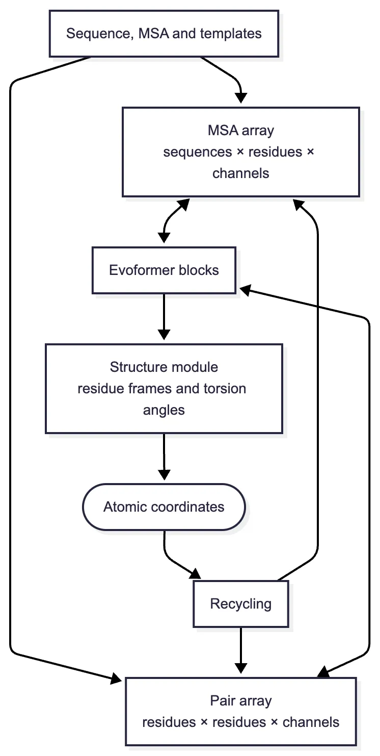
Training required more than a large architecture and its losses. The supervised examples came from experimentally determined PDB structures, but each training step sampled only a crop of residues and a subset of MSA rows so that proteins and alignments of different sizes could fit in memory. The published system also used self-distillation: an earlier model predicted structures for a large collection of sequences, confident predictions were treated as additional training targets, and the final network learned from a mixture of experimental and predicted examples.² This mixture helped data efficiency, but it also means that the training distribution reflects what was deposited in the PDB and what an earlier predictor considered plausible—not every condition or conformation a protein can occupy.

Why CASP14 was a change of regime

At CASP14 in 2020, AlphaFold2 achieved near-experimental backbone accuracy for many targets and a large advantage over other submissions.² The phrase “near experimental” needs context. Experimental structures also contain uncertainty, and agreement varies by region and target. Nonetheless, the performance was high enough that predicted structures could become practical starting points for many biological investigations rather than speculative models used only when no alternative existed.

The achievement is sometimes described as “solving protein folding.” That phrase combines several different problems. AlphaFold2 predicts a likely static structure from sequence and evolutionary context. It does not ordinarily simulate the physical path by which the chain folds, calculate folding rates, produce a thermodynamically weighted ensemble, or specify how pH, temperature, membranes, modifications, and binding partners reshape the landscape. It solved an important prediction problem for a broad class of proteins, which is both more precise and more useful than the larger slogan.

How RoseTTAFold arrived at a related idea

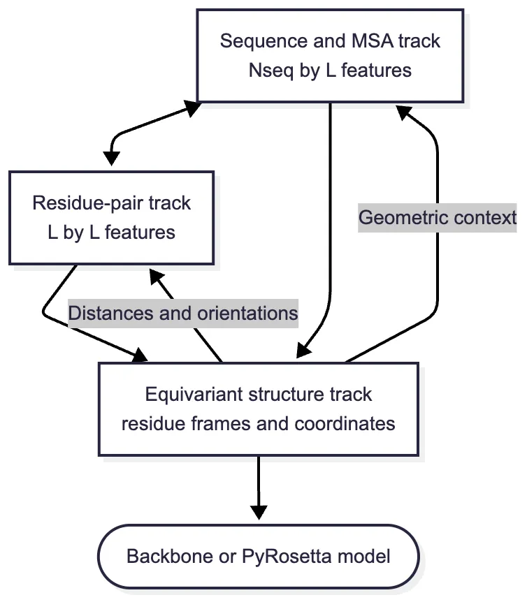
RoseTTAFold grew out of an unusually compressed period of architectural experimentation. After AlphaFold2’s CASP14 results were presented but before its implementation was published, Minkyung Baek, Frank DiMaio, David Baker, and colleagues at the University of Washington asked which reported ideas could be independently reconstructed for structural biology and protein design.⁴ They first built a two-track network that repeatedly exchanged information between an MSA representation and a residue-pair map. They then reasoned that coordinates should participate in this exchange rather than appear only after the sequence and pair calculations were complete. The resulting three-track architecture was a convergent response to the same integration problem, not a copy of the later published AlphaFold2 code.

The three tracks stored different kinds of arrays. The sequence track held a learned vector for every residue in every selected MSA row, approximately $N_{seq}\times L\times c_1.$ The pair track held a vector for every query-residue pair, $L\times L\times c_2,$ encoding proposed distances, orientations, and relational context. The structure track held three-dimensional backbone coordinates and features attached to residues. These are not three independent predictions. They are three resolutions of one developing hypothesis about the protein.

The three-track cycle can be summarized without treating the tracks as black boxes. If $M^{(\ell )},$ $Z^{(\ell )},$ and $X^{(\ell )}$ denote the sequence, pair, and coordinate states at stage $\ell ,$ then a schematic update is

Attention along MSA rows and columns performs part of $F_M,$ allowing sequence positions to exchange evolutionary evidence. Sequence-derived information enters $F_Z,$ while the geometric summary $G(X)$—including distances and orientations calculated from provisional coordinates—writes the current three-dimensional hypothesis back into pair reasoning. The coordinate map $F_X$ then treats residues as nodes in a geometric graph and uses the updated sequence and pair features to move them. The equations are schematic because each map contains several attention, projection, and normalization layers; their purpose is to show that no track is merely an output head. Each becomes an input to the others.

The coordinate map uses an SE(3)-equivariant transformer. If $QX+𝐭$ means applying the same three-dimensional rotation $Q$ and translation $𝐭$ to all input coordinates, equivariance requires

Thus rotating the input rotates the predicted structure, and translating the input translates it; the network does not have to relearn the same protein from every camera angle. This differs subtly from an invariant scalar output, which would remain numerically unchanged. Distances used by the other tracks are invariant, while coordinate outputs must be equivariant. Because geometry returns through $G(X),$ an impossible three-dimensional arrangement can alter the next round of sequence and pair reasoning.⁴

This circulation occurred in stages because a full three-track calculation was expensive. RoseTTAFold used many two-track blocks for sequence–pair reasoning and a smaller number of three-track blocks for coordinate updates. Hardware memory also limited training on complete large proteins. The team trained with discontinuous crops containing two separated sequence segments and 260 residues in total, teaching the model about long-range contacts while keeping the arrays manageable. At inference, overlapping crop predictions could be combined.

The original release offered two routes from the learned representations to a final structure. A lower-memory route converted predicted distance and orientation distributions into restraints for PyRosetta, which assembled and refined an all-atom model. The end-to-end route sent averaged one- and two-dimensional features through a final equivariant layer to predict backbone coordinates directly. Its training objective can be organized schematically as

The six-dimensional geometry term supervises binned distances and orientations between residue pairs, the coordinate term supervises the equivariant structure output, and the accuracy term teaches a residue-level confidence estimate. Their gradients propagate through the connected tracks, so a coordinate error can change how sequence and pair features are learned. The first inference route retained a classical structure-building engine; the second demonstrated that the neural network itself could be trained from sequence to coordinates.⁴

The architecture was tested as more than a CASP score. The authors used predictions to help solve X-ray crystallography and cryogenic electron microscopy structures, model previously uncharacterized proteins, and infer protein complexes directly from sequence rather than predicting subunits and docking them afterward. RoseTTAFold was generally less accurate than AlphaFold2 on difficult monomers, and its crop-and-assembly procedure, MSA dependence, and residue-level chemistry remained important constraints. Its source code and parameters were nevertheless released, and the three-track organization was readily modified inside a laboratory already joining computation with experimental design.

RoseTTAFold’s historical role therefore extends beyond its initial benchmark. RFjoint Inpainting first adapted its network to complete backbones around fixed functional motifs in one step. RFdiffusion then turned the structure track into an iterative denoiser capable of sampling diverse new backbones. RoseTTAFoldNA and RoseTTAFold All-Atom widened the molecular alphabet to nucleic acids, ligands, metals, and modifications. A predictor trained to organize structural possibilities became a reusable geometric engine for generation and heterogeneous molecular modelling.

This is one reason scientific influence cannot be read from a single accuracy table. AlphaFold2 established the dominant practical standard for prediction. RoseTTAFold established an open and experimentally connected architectural lineage whose descendants changed what could be designed.

How AlphaFold2 became a family and infrastructure

Once inference became reliable and reasonably automated, the unit of work changed. The question was no longer only whether a difficult protein could be modelled; it was whether entire proteomes could be covered. AlphaFold predictions were produced for most of the human proteome,⁵ and the AlphaFold Protein Structure Database expanded to hundreds of millions of sequences.⁶ ESMFold later pushed predicted structural coverage still further through faster single-sequence inference.

A proteome is the complete set of proteins encoded or produced by a cell, organism, or biological sample. Moving from one carefully studied target to a proteome changes the practical problem: manual inspection is no longer possible for every prediction, naming and database links must be automated, and calibrated confidence becomes essential for deciding which regions are usable without expert reconstruction.

Complex prediction expanded in parallel. AlphaFold-Multimer modified the training mixture and representation of chains to model protein assemblies.⁷ ColabFold made alignment search and inference accessible to a much wider group of users. OpenFold reproduced AlphaFold2 training in an open framework, permitting experiments that require more than inference code, such as retraining, ablation, and controlled studies of generalization.⁸

These projects have different relationships to AlphaFold2. AlphaFold-Multimer is a direct model extension from the same research lineage. It retains the AlphaFold2 trunk and structure logic but tells the network which residues belong to which chain, which chains are chemically identical, and which copies are symmetry-related. Relative-position features prevent the end of one chain from being mistaken for a peptide-bonded neighbour of the next. The input combines unpaired alignments for individual chains with paired rows that attempt to place interacting homologues from the same organism together. Training on multimeric PDB examples and adding interface-sensitive confidence and ranking terms made inter-chain geometry a primary objective rather than a side effect.⁷

Multimer training also has to resolve a mathematical ambiguity absent from most single-chain examples. If a complex contains identical or interchangeable chains, the labels assigned to those chains in a PDB file are arbitrary: swapping two copies does not create a different physical assembly, but a naive residue-by-residue loss could treat it as a large error. AlphaFold-Multimer therefore matches the predicted chains to the target chains before evaluating the structural loss. Abstractly, it chooses ${\displaystyle {\pi }^{*}=\underset{\pi \in \Pi }{\mathrm{a}\mathrm{r}\mathrm{g}\mathrm{m}\mathrm{i}\mathrm{n}{\mathcal{L}}_{\mathrm{s}\mathrm{t}\mathrm{r}\mathrm{u}\mathrm{c}\mathrm{t}\mathrm{u}\mathrm{r}\mathrm{e}}(\hat{X},\pi (X^{*})),}}$ where $\Pi$ is the set of chemically valid target-chain assignments and $\pi (X^{*})$ is the experimental structure with those labels permuted. The equation expresses the underlying problem; the implementation uses an efficient chain-assignment procedure rather than enumerating every possible permutation.

The ranking score likewise separates confidence in the overall fold from confidence in the interface: for example, ranking confidence ${\displaystyle =0.8\mathrm{i}\mathrm{p}\mathrm{T}\mathrm{M}+0.2\mathrm{p}\mathrm{T}\mathrm{M}.}$ Predicted TM score (pTM) summarizes expected global topology from the predicted aligned-error distribution. Interface predicted TM score (ipTM) emphasizes residue pairs that cross chain boundaries. A model can therefore have confident monomer folds but an uncertain assembly, producing a high pTM and lower ipTM; the weighted ranking score deliberately makes that interface uncertainty dominant.⁷

Those additions solved an important representation problem, but not every assembly problem. The user must normally specify the chain identities and stoichiometry—the number of copies of each component. Incorrect MSA pairing can invent or erase evolutionary evidence for an interface. Transient interactions, alternative oligomeric states, antibodies, and complexes without strong coevolution remain uneven. AlphaFold3 later followed this direct lineage while replacing several of its central components to accommodate proteins, nucleic acids, ligands, ions, and modifications together.⁹

ColabFold belongs to the access layer. It combines MMseqs2-based sequence search with AlphaFold2, AlphaFold-Multimer, or RoseTTAFold inference, reducing the alignment-search bottleneck and packaging the workflow for local servers and Google Colaboratory. Its original report measured a 40- to 60-fold faster search and close to one thousand predictions per day on a one-GPU server under the reported settings.¹⁰ ColabFold did not become useful by retraining a new folding architecture; it changed who could run the architecture, how quickly its inputs could be assembled, and how easily many predictions could be launched.

OpenFold belongs to the reproducibility layer. It is an independent open implementation and training effort rather than a later DeepMind checkpoint. Reproducing the data pipeline, losses, distributed training, and numerical behaviour made it possible to ask questions that released inference code alone could not answer: whether the system could be retrained from public resources, which components mattered in ablations, and how training choices affected generalization.⁸ The AlphaFold Database is different again: it is deployment at archive scale, turning model outputs into a searchable scientific resource rather than changing the neural architecture.⁶

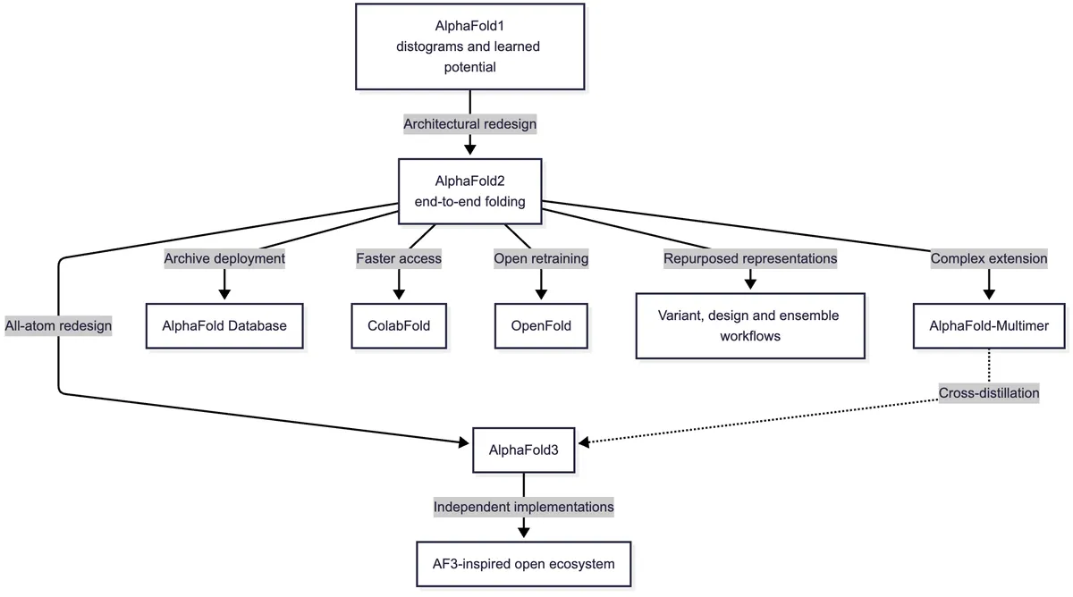
The last two branches are scientific adaptations rather than numbered AlphaFold releases. AlphaMissense reuses learned structural context for variant classification; BindCraft optimizes binder sequences through AlphaFold2; altered MSA sampling elicits alternative conformations; and BioEmu uses a simplified frozen AlphaFold2 sequence encoder to condition an ensemble generator. The AlphaFold3-inspired open ecosystem—discussed in the article on molecular assemblies—similarly consists of independent implementations and extensions, not one official sequence of numbered descendants.

These developments created three layers of infrastructure: models that could be run, databases of predictions that could be queried, and open implementations that could be altered. The distinction matters. Access to a server allows use; access to weights allows local inference; access to training code and data provenance allows deeper scientific inspection.

Where static prediction remains conditional

AlphaFold2 performs best when the target resembles the distribution represented by natural sequences and experimental structures. Intrinsically disordered regions do not have one stable folded answer. Antibody loops, flexible peptides, novel complexes, membrane contexts, and alternative conformations can be difficult. A model may also predict an isolated chain differently from the same chain bound to a partner.

Researchers have found that clustering an MSA and altering sampling can elicit some alternative known states from AlphaFold2.¹¹ This shows that the network contains information beyond its default output, but it does not turn confidence values into equilibrium populations. The predicted alternatives are samples from a model under a modified procedure, not automatically a thermodynamic ensemble.

The deeper limitation is that structure sits between sequence and biological behaviour. Coordinates can suggest an active site, interface, or mutation mechanism, but they do not directly specify concentrations, kinetics, cellular localization, expression, toxicity, or phenotype. AlphaFold2 made the structural layer far more accessible; its success made the neighbouring unsolved layers more visible.

Why this advance enabled generation

End-to-end predictors learned reusable representations of what protein-like geometry looks like. Once those representations existed, researchers could use them in reverse. They could optimize a sequence until a predictor became confident, condition a model on a desired backbone, or retrain a structure network to reverse added noise.

Before following that generative turn, however, another lineage must be introduced. Protein language models learned from sequence databases without constructing an explicit MSA for every query. They offered a different way to compress evolutionary history and eventually joined sequence, structure, and function in one generative system.

References

#Biology

References

AlQuraishi, M. (2019). End-to-end differentiable learning of protein structure. Cell Systems, 8(4), 292–301.e3. https://doi.org/10.1016/j.cels.2019.03.006↩
Jumper, J., Evans, R., Pritzel, A., Green, T., Figurnov, M., Ronneberger, O., et al. (2021). Highly accurate protein structure prediction with AlphaFold. Nature, 596(7873), 583–589. https://doi.org/10.1038/s41586-021-03819-2↩
Senior, A. W., Evans, R., Jumper, J., Kirkpatrick, J., Sifre, L., Green, T., et al. (2020). Improved protein structure prediction using potentials from deep learning. Nature, 577(7792), 706–710. https://doi.org/10.1038/s41586-019-1923-7↩
Baek, M., DiMaio, F., Anishchenko, I., Dauparas, J., Ovchinnikov, S., Lee, G. R., et al. (2021). Accurate prediction of protein structures and interactions using a three-track neural network. Science, 373(6557), 871–876. https://doi.org/10.1126/science.abj8754↩
Tunyasuvunakool, K., Adler, J., Wu, Z., Green, T., Zielinski, M., Žídek, A., et al. (2021). Highly accurate protein structure prediction for the human proteome. Nature, 596(7873), 590–596. https://doi.org/10.1038/s41586-021-03828-1↩
Varadi, M., Anyango, S., Deshpande, M., Nair, S., Natassia, C., Yordanova, G., et al. (2022). AlphaFold Protein Structure Database: Massively expanding the structural coverage of protein-sequence space with high-accuracy models. Nucleic Acids Research, 50(D1), D439–D444. https://doi.org/10.1093/nar/gkab1061↩
Evans, R., O’Neill, M., Pritzel, A., Antropova, N., Senior, A., Green, T., et al. (2021). Protein complex prediction with AlphaFold-Multimer. bioRxiv. https://doi.org/10.1101/2021.10.04.463034↩
Ahdritz, G., Bouatta, N., Floristean, C., Kadyan, S., Xia, Q., Gerecke, W., et al. (2024). OpenFold: Retraining AlphaFold2 yields new insights into its learning mechanisms and capacity for generalization. Nature Methods, 21(8), 1514–1524. https://doi.org/10.1038/s41592-024-02272-z↩
Abramson, J., Adler, J., Dunger, J., Evans, R., Green, T., Pritzel, A., et al. (2024). Accurate structure prediction of biomolecular interactions with AlphaFold 3. Nature, 630(8016), 493–500. https://doi.org/10.1038/s41586-024-07487-w↩
Mirdita, M., Schütze, K., Moriwaki, Y., Heo, L., Ovchinnikov, S., & Steinegger, M. (2022). ColabFold: Making protein folding accessible to all. Nature Methods, 19(6), 679–682. https://doi.org/10.1038/s41592-022-01488-1↩
Wayment-Steele, H. K., Ojoawo, A., Otten, R., Apitz, J. M., Pitsawong, W., Hömberger, M., et al. (2024). Predicting multiple conformations via sequence clustering and AlphaFold2. Nature, 625(7996), 832–839. https://doi.org/10.1038/s41586-023-06832-9↩