Predicting and designing proteins (2): How evolution became a source of structural information

14 Jul, 2026

Imagine comparing the same sentence as it has been copied and edited in many communities for millions of years. Some words change freely. Others remain nearly fixed because changing them destroys the meaning. A third group changes in pairs: when one word is replaced, another tends to change as well because the two must remain compatible. Protein families leave a record with a related structure. Their sequences are not sentences, and evolution is not an author, but patterns of conservation and coordinated substitution contain information about molecular constraints.

This insight changed structure prediction because it supplied evidence about residues that are far apart in the written sequence but close together in three-dimensional space. It also created the immediate technical ancestry of AlphaFold: first infer contacts and distances from evolutionary variation, then learn how those geometric constraints fit together.

From relatives to alignments

Proteins related by descent are homologues. To compare them, researchers construct a multiple sequence alignment (MSA), arranging the sequences in rows so that columns represent positions believed to share an evolutionary origin. Insertions and deletions create gaps. A deeply sampled family may contain thousands of aligned sequences; a rare or recently evolved protein may have few.

DNA is the hereditary molecule whose ordered chemical units store biological information. A gene is a region of DNA that cells can use, through an intermediate RNA copy, to specify a protein sequence. The variations arise because DNA is copied from one generation to the next with occasional changes. Some changes alter the encoded amino acid; if the resulting protein remains compatible with survival and reproduction, that version may persist in descendants. An alignment is an attempt to place the residues inherited from the same ancestral position in one column, even after different lineages have inserted or deleted residues. It is therefore a historical hypothesis as well as a rectangular data table.

An MSA contains several kinds of signal. A highly conserved column suggests that few substitutions are tolerated. A variable column suggests greater freedom. If substitutions at two columns are correlated, the positions may be functionally or structurally coupled. For example, replacing a large side chain with a smaller one on one side of a protein core may favour a compensating change nearby.

The tempting method is to calculate covariance between every pair of columns. The result is useful but confounded. Closely related species share substitutions because of common ancestry, not necessarily because two residues touch. Indirect correlations also proliferate: if position A interacts with B and B interacts with C, then A and C may appear correlated even without direct contact.

How direct coupling analysis separated interactions

During the late 2000s and early 2010s, researchers drew on statistical physics to fit global models to whole alignments. Instead of asking whether two columns vary together in isolation, these models asked which set of direct pairwise couplings could jointly explain the observed family. Message-passing and maximum-entropy approaches showed that the strongest inferred direct couplings were enriched for residue contacts.¹²

“Global” means that all positions are considered in one model, so the explanation assigned to one pair depends on the alternatives available elsewhere. The maximum-entropy principle chooses the least-committal probability distribution that still reproduces selected observations from the alignment. In practical terms, the model tries not to invent extra structure: it adds pairwise dependencies only to the extent needed to account for the observed patterns. This is how a correlation transmitted through B can be separated, imperfectly, from a more direct A–C dependency.

This family of methods became known as direct coupling analysis (DCA). The word “direct” is important: it refers to separating a putative A–B relationship from correlations mediated through the rest of the sequence. The output is not a measured physical force. It is a statistical parameter whose magnitude can serve as evidence that two positions have constrained one another during evolution.

Debora Marks, Chris Sander, and colleagues then asked whether the inferred contacts were sufficient to build complete structures. EVfold converted high-scoring evolutionary couplings into spatial restraints and used them to calculate three-dimensional models.³ Related work applied the approach to membrane proteins, a class for which experimental structures were especially sparse.⁴ The conceptual achievement was striking: natural selection had perturbed related sequences across geological time, and a statistical model could read the accumulated outcomes as an approximate structural experiment.

The approach also had a clear requirement. To estimate couplings, a family needs enough diverse sequences. Ten thousand nearly identical sequences contain less useful information than a smaller set distributed across evolutionary distance. Sequence count, diversity, alignment quality, and family boundaries all affect the signal.

What the coupling matrices contained

A common mathematical form for direct coupling analysis is a Potts model. For an aligned sequence $s,$ it assigns an energy-like score ${\displaystyle E(s)=\sum _i{h}_i(s_i)+\sum _{i<j}{J}_{ij}(s_i,s_j).}$ The first term, $h_i,$ records which amino acids are individually favoured at position $i.$ The second, $J_{ij},$ records which pairs of amino acids are compatible at positions $i$ and $j$ after the rest of the alignment has been considered. For the twenty standard amino acids, every position pair therefore has roughly a $20\times 20$ block of coupling values. A strong block says more than “these columns correlate”: it specifies, for example, that a bulky residue at one position is statistically paired with a small residue at the other.

Fitting all these numbers is difficult because an alignment supplies far fewer independent examples than its row count suggests. Three related safeguards address different versions of this problem. The formulas below are schematic—specific DCA implementations differ—but they make the purpose of each safeguard concrete.

First, nearly identical sequences are down-weighted. Let $s^{(m)}$ be row $m$ of an alignment containing $M$ sequences. A common rule assigns

${\displaystyle w_m=\frac{1}{{\displaystyle \sum _{n=1}^M\mathbf{1}[id(s^{(m)},s^{(n)})\ge \theta ]}},M_{\mathrm{e}\mathrm{f}\mathrm{f}}=\sum _{m=1}^M{w}_m.}$

Here, $id$ is sequence identity, $\theta$ is a similarity threshold, and the indicator $\mathbf{1}[·]$ equals one when its condition is true. If one sequence has 99 near-duplicates, each of those 100 rows receives a weight near $1/100,$ so together they contribute roughly one effective sequence. An isolated sequence receives a weight near one. The effective count $M_{\mathrm{e}\mathrm{f}\mathrm{f}}$ therefore measures diversity more usefully than the raw number of rows, although it does not make the remaining sequences truly independent.

Second, pseudocounts prevent finite data from being interpreted as absolute impossibility. Suppose $f_{ij}(a,b)$ records how often amino acids $a$ and $b$ occur together at positions $i$ and $j.$ With $q$ possible residue symbols and a total pseudocount strength $\alpha ,$ one simple smoothed estimate is

${\displaystyle {\tilde{f}}_{ij}(a,b)=\frac{{\displaystyle \sum _m{w}_m\mathbf{1}[s_i^{(m)}=a,s_j^{(m)}=b]+\alpha /q^2}}{M_{\mathrm{e}\mathrm{f}\mathrm{f}}+\alpha }.}$

Without the $\alpha /q^2$ term, an unobserved pair has estimated frequency zero. Logarithms of that frequency can diverge, and covariance calculations can become singular or unstable. The pseudocount gives every possible pair a small nonzero baseline. It does not claim that an unseen combination was observed; it expresses the more cautious conclusion that a finite alignment cannot prove its probability is exactly zero. A larger $\alpha$ produces more smoothing and therefore trusts the observed counts less.

Third, regularization acts on the fitted parameters rather than the counts. A common quadratic or $L_2$ form estimates the fields and couplings by minimizing an objective such as

${\displaystyle (\hat{h},\hat{J})=\underset{h,J}{\mathrm{a}\mathrm{r}\mathrm{g}\mathrm{m}\mathrm{i}\mathrm{n}}[-\ell (h,J)+{\lambda }_h\sum _{i,a}{h}_i(a{)}^2+{\lambda }_J\sum _{i<j,a,b}{J}_{ij}(a,b{)}^2],}$

where $\ell$ is the log-likelihood of the alignment and the $\lambda$ values control the penalty. A large coupling is retained only if it improves the fit enough to overcome that penalty; couplings supported mainly by sampling noise are pulled toward zero. Excessive regularization can erase real signal, while too little lets the millions of $J_{ij}(a,b)$ values memorize a sparse alignment.

The three operations are therefore not interchangeable: weighting limits duplicated evolutionary evidence, pseudocounts stabilize empirical frequencies, and regularization limits the complexity of the fitted explanation. Early message-passing methods and later inverse-covariance or pseudolikelihood approximations made the global fit computationally manageable.¹²⁵ These implementation choices are part of the biological inference: without them, phylogenetic duplication, finite sampling, and uneven family coverage can look like physical contact.

The resulting model still did not directly contain atomic coordinates. It assigned a $q\times q$ coupling block $J_{ij}$ to every position pair, so investigators first had to compress that block into one number. A widely used choice, after putting the couplings into a consistent gauge and usually omitting the alignment-gap state, is the Frobenius norm:⁵

${\displaystyle F_{ij}=\Vert J_{ij}{\Vert }_F={(\sum _{a,b}{J}_{ij}(a,b{)}^2)}^{1/2}.}$

Squaring prevents positive and negative entries from cancelling. A large $F_{ij}$ can therefore reflect one exceptionally strong amino-acid pairing or many moderately strong pairings. The compression is useful for ranking, but it discards which particular residue combinations produced the score. Different numerical $h$ and $J$ tables can represent the same Potts probability distribution; a gauge is the convention used to select one standardized table from these equivalent parameterizations before their norms are compared.

Raw norms also inherit broad background effects. If position $i$ is variable or noisy enough to score highly with many other positions, every pair involving $i$ can be inflated. The commonly used average-product correction (APC) subtracts the score expected from those row and column tendencies:⁵ ${\displaystyle F_{ij}^{\mathrm{A}\mathrm{P}\mathrm{C}}=F_{ij}-\frac{{\bar{F}}_{i·}{\bar{F}}_{·j}}{{\bar{F}}_{··}},}$ where ${\bar{F}}_{i·}$ and ${\bar{F}}_{·j}$ are the mean scores involving positions $i$ and $j,$ and ${\bar{F}}_{··}$ is the mean over position pairs. A pair remains high after APC only when its coupling is stronger than expected from the general tendency of each position to couple with others. Some DCA variants instead summarize a block through direct information, which measures the two-position dependency implied by the direct coupling. The exact score differs, but the purpose is the same: turn a matrix of amino-acid-specific relationships into a scalar that can order position pairs.²

Investigators ranked pairs by such corrected scores, often excluding positions close together along the sequence, and treated the strongest long-range pairs as probable contacts. The score was evidence for contact, not a calibrated probability that contact must occur. High-ranking pairs could restrain a separate folding calculation, but a false restraint could distort the whole fold. Sparse families created another failure mode: if there were not enough diverse sequences, the millions of coupling parameters could not be estimated reliably. Metagenomic sequencing helped not by changing the equation, but by supplying many more natural experiments in which evolution had tried different residue combinations.

Why metagenomics improved structure prediction

Traditional sequence databases were built largely from organisms that scientists could isolate, culture, or sequence individually. Metagenomics instead sequences genetic material collected from an environment such as seawater, soil, or the human gut. It revealed immense numbers of proteins from organisms that had never been cultivated.

For structure prediction, this expansion did more than add new targets. It filled previously shallow alignments with additional relatives. Sergey Ovchinnikov and colleagues combined metagenomic sequence information, coupling-derived restraints, and Rosetta modelling to predict structures across hundreds of protein families.⁶ The work demonstrated an unusual scaling relationship: better structural coverage could come from collecting more sequences, even without collecting a corresponding experimental structure for every family.

The improvement also revealed a bias that continues into modern models. Proteins from large, well-sampled families are easier to model with explicit evolutionary statistics than orphan proteins with few known relatives. A method’s average benchmark score can therefore conceal substantial differences in difficulty.

How neural networks learned the shape of contact maps

DCA produces a matrix of pairwise scores. If a protein has 200 residues, the matrix has 200 rows and 200 columns; a high value at row 25 and column 140 suggests a relationship between those positions. A binary contact map labels pairs that lie within a chosen distance in the experimental structure.

Contact maps have patterns. Alpha helices and beta sheets produce characteristic lines and bands. Residues participate in networks of interactions that are not independent pairwise events. Researchers therefore began treating contact prediction as a supervised pattern-recognition problem rather than ranking every pair independently.

MetaPSICOV, developed by David Jones and colleagues, was an important intermediate system because it treated several imperfect methods as complementary evidence.⁷ Its inputs included PSICOV and other coevolution scores, sequence profiles, predicted secondary structure and solvent accessibility. A first neural network estimated contacts from a local window of these features; a second stage examined the preliminary contact map together with a wider neighbourhood and corrected predictions that did not fit the surrounding pattern. This meta-prediction strategy—learning when several predictors should reinforce or overrule one another—substantially improved long-range contact accuracy without pretending that any one coupling statistic was sufficient.

RaptorX-Contact, developed by Sheng Wang, Jinbo Xu, and colleagues, pushed the same idea into much deeper networks.⁸ One-dimensional features such as sequence profiles were first processed along the chain and then converted into two-dimensional features for every residue pair. They were joined with pairwise coevolution information in an $L\times L\times C$ tensor. Dozens of residual convolutional layers then passed information across the square map. A residual connection adds a layer’s input to its transformed output, which lets very deep networks refine a representation without having to reconstruct it at every layer. The model could therefore judge a candidate contact in the context of extended sheet patterns and other contacts far away in the matrix.

The achievement was especially important for proteins with hundreds of sequence relatives rather than thousands: supervised structural patterns could partly compensate for imperfect coevolution. The limitations also became clearer. A binary contact label discarded distance and orientation; a full $L\times L$ tensor consumed memory quadratically as proteins grew; and the network still handed its answer to a separate folding procedure. Deep contact prediction improved the evidence supplied to folding without yet integrating the folding calculation itself.

From contacts to distances and orientations

A contact says that two residues are near one another under a chosen threshold. That discards useful information. Two residues separated by 6 ångströms and two separated by 11 ångströms may both be labelled contacts even though the geometrical implications differ. A distogram instead assigns a probability distribution over distance ranges for every residue pair.

An ångström is one ten-billionth of a metre, a convenient unit at atomic scale; a typical carbon–carbon bond is roughly 1.5 ångströms long. A distogram does not insist that one distance is certainly correct. It might assign, for example, most probability to 6–8 ångströms and smaller probabilities to neighbouring ranges. Preserving that uncertainty gives the later coordinate-building step room to reconcile thousands of imperfect constraints.

How AlphaFold1 learned a protein-specific potential

DeepMind’s CASP13 system was published simply as AlphaFold. “AlphaFold1” is a retrospective name used to distinguish it from the fundamentally redesigned AlphaFold2. The first system deserves that distinction because it was more than an early version of the later network. It supplied a new answer to a specific question: if evolution and a neural network can estimate uncertain residue-pair geometry, how can those estimates become an energy-like surface over complete structures?⁹

The computation began with a query sequence and related sequences found by HHblits and PSI-BLAST in Uniclust30 and the non-redundant sequence database. From the MSA, the pipeline constructed one-dimensional features for individual positions and two-dimensional features for residue pairs, including coevolutionary statistics. For a protein of length $L,$ these pair features formed an $L\times L\times C$ array, where $C$ denotes the feature channels stored for each pair. A very deep residual convolutional network processed that square array. Dilated convolutions allowed a layer to gather information across increasingly wide regions of the pair map, while residual connections allowed a deep stack to be trained without losing the learning signal through its many layers.⁹

For every residue pair, the network output a distribution over 64 distance intervals rather than one coordinate or one contact label. A separate output predicted backbone torsion distributions. The distance probabilities were compared with a reference distribution expected without sequence-specific evidence and converted into a potential of mean force, schematically ${\displaystyle U_{ij}(d)=-\log {\displaystyle \frac{P_{ij}(d)}{P_{\mathrm{r}\mathrm{e}\mathrm{f}}(d)}}.}$ Here, $P_{ij}(d)$ is the network’s probability that residues $i$ and $j$ have separation $d,$ while $P_{\mathrm{r}\mathrm{e}\mathrm{f}}(d)$ describes how common that distance is in a generic background. A distance that the network considers unusually plausible receives a favourable contribution; one that is less plausible than the background receives a penalty. Summing these learned pair terms with torsion and stereochemical terms creates a different objective function for every query protein.

Structure realization was still a separate calculation. Starting from candidate conformations, gradient-based optimization changed structural variables to lower the learned potential, with noisy restarts exploring more than one basin; selected structures could then receive Rosetta relaxation. The network did not watch this search and revise its distogram when the resulting three-dimensional geometry exposed a contradiction. Information crossed the network–optimizer boundary only once.⁹

The training structures came from a dated PDB and were split by CATH structural domains; sequence features used dated releases of Uniclust30 and the PSI-BLAST non-redundant database. These cutoffs matter because they define what counted as unseen during CASP13. On the blind free-modelling targets, AlphaFold produced high-accuracy structures for 24 of 43 domains by the paper’s TM-score criterion, compared with 14 for the next-best system.⁹ That result established learned distance distributions as a stronger structural representation than binary contacts and showed that a learned potential could guide comparatively simple gradient optimization.

Its remaining weaknesses were equally formative. Accuracy still depended on MSA information, the pair array grew quadratically with sequence length, probability calibration affected the potential, and coordinate search required repeated optimization after the neural network had finished. AlphaFold1 conquered the information bottleneck more convincingly than the integration bottleneck. AlphaFold2 was built around removing that remaining separation.

The Baker group’s trRosetta completed another part of this transition.¹⁰ Its deep two-dimensional residual network predicted distributions for one inter-residue distance and three relative-orientation angles. Distance constrains how far apart two residues are; orientation specifies how the local backbone frames face one another. This reduces ambiguity in the same way that knowing both the distance and bearing to a landmark is more informative than knowing distance alone.

Each predicted distribution was converted into a smooth restraint for Rosetta. Rosetta then changed backbone torsions and rigid-body relationships to find coordinates that jointly satisfied the learned restraints, followed by all-atom refinement. The model could also be used in reverse: optimize a sequence so that trRosetta predicted a confident, internally consistent geometry. That possibility helped establish network hallucination, in which a predictor’s learned notion of protein-like structure becomes an objective for generation. trRosetta therefore sits at a historical junction. It was still a modular predictor-plus-search pipeline, but its orientation-aware geometry fed directly into both RoseTTAFold’s end-to-end predictor and early learned design methods.

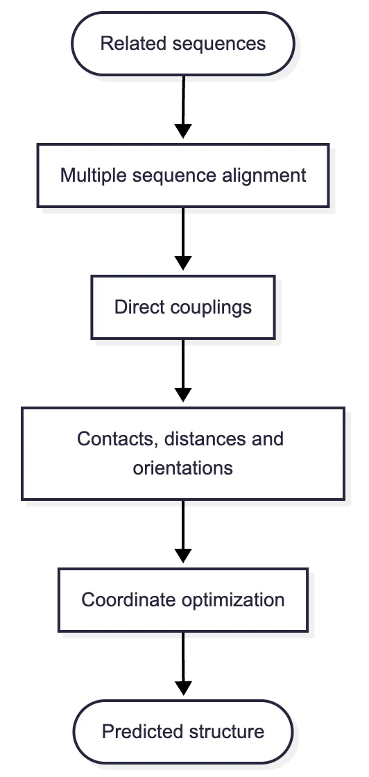
What evolution could and could not provide

By 2020, the field had learned how to convert sequence databases into strong geometric evidence. This was not a minor preprocessing improvement. It altered the nature of experimental data: every newly sequenced organism could contribute constraints to protein families whose structures had never been measured.

Yet the pipeline still had seams. Alignment construction, feature extraction, restraint prediction, and coordinate optimization were separately engineered stages. Errors accumulated between them. The learned network reasoned mainly over a two-dimensional residue-pair representation, while the final coordinates were produced elsewhere. Shallow alignments remained difficult, and the procedure could be computationally expensive at query time.

The next generation of models removed that boundary. Rather than predict restraints and hand them to an external search, AlphaFold2 and RoseTTAFold allowed sequence, pairwise relationships, and coordinates to update one another repeatedly inside a trainable system. End-to-end prediction was not the rejection of coevolution; it was its integration into a larger geometrical computation.

Onto the next article.

References

#Biology

References

Weigt, M., White, R. A., Szurmant, H., Hoch, J. A., & Hwa, T. (2009). Identification of direct residue contacts in protein–protein interaction by message passing. Proceedings of the National Academy of Sciences, 106(1), 67–72. https://doi.org/10.1073/pnas.0805923106↩
Morcos, F., Pagnani, A., Lunt, B., Bertolino, A., Marks, D. S., Sander, C., et al. (2011). Direct-coupling analysis of residue coevolution captures native contacts across many protein families. Proceedings of the National Academy of Sciences, 108(49), E1293–E1301. https://doi.org/10.1073/pnas.1111471108↩
Marks, D. S., Colwell, L. J., Sheridan, R., Hopf, T. A., Pagnani, A., Zecchina, R., & Sander, C. (2011). Protein 3D structure computed from evolutionary sequence variation. PLoS ONE, 6(12), e28766. https://doi.org/10.1371/journal.pone.0028766↩
Hopf, T. A., Colwell, L. J., Sheridan, R., Rost, B., Sander, C., & Marks, D. S. (2012). Three-dimensional structures of membrane proteins from genomic sequencing. Cell, 149(7), 1607–1621. https://doi.org/10.1016/j.cell.2012.04.012↩
Ekeberg, M., Lövkvist, C., Lan, Y., Weigt, M., & Aurell, E. (2013). Improved contact prediction in proteins: Using pseudolikelihoods to infer Potts models. Physical Review E, 87(1), 012707. https://doi.org/10.1103/PhysRevE.87.012707↩
Ovchinnikov, S., Park, H., Varghese, N., Huang, P.-S., Pavlopoulos, G. A., Kim, D. E., et al. (2017). Protein structure determination using metagenome sequence data. Science, 355(6322), 294–298. https://doi.org/10.1126/science.aah4043↩
Jones, D. T., Singh, T., Kosciolek, T., & Tetchner, S. (2015). MetaPSICOV: Combining coevolution methods for accurate prediction of contacts and long range hydrogen bonding in proteins. Bioinformatics, 31(7), 999–1006. https://doi.org/10.1093/bioinformatics/btu791↩
Wang, S., Sun, S., Li, Z., Zhang, R., & Xu, J. (2017). Accurate de novo prediction of protein contact map by ultra-deep learning model. PLOS Computational Biology, 13(1), e1005324. https://doi.org/10.1371/journal.pcbi.1005324↩
Senior, A. W., Evans, R., Jumper, J., Kirkpatrick, J., Sifre, L., Green, T., et al. (2020). Improved protein structure prediction using potentials from deep learning. Nature, 577(7792), 706–710. https://doi.org/10.1038/s41586-019-1923-7↩
Yang, J., Anishchenko, I., Park, H., Peng, Z., Ovchinnikov, S., & Baker, D. (2020). Improved protein structure prediction using predicted interresidue orientations. Proceedings of the National Academy of Sciences, 117(3), 1496–1503. https://doi.org/10.1073/pnas.1914677117↩